Summary
Creating bounding volume hierarchies for triangle meshes in parallel on multi-core CPU platforms.
Background
- Creating a bounding volume hierarchy is often quite an expensive process for arbitrarily complex meshes. It is in essence a process of hierarchically sorting the scene primitives into spatially local groups.
- The serial algorithm involves iteratively dividing the set of scene primitives, where the best division is dependent on a cost function known as the surface area heuristic (SAH). The end product is a binary tree, where nodes represent a bounding box surrounding all scene primitives contained in the leaves of the subtree with the current node as its root. While leaf nodes represent a list of scene primitives.
- The process of creating a BVH can be split into many sub problems. Viewing each node of the BVH tree as a sub problem already puts into view the potential for parallelism.
- Since sequential creation of BVHs can be expensive, it involves at least O(nlogn) since sorting can be reduced to the problem of BVH creation (at least when the BVH can have arbitrary depth and leaf nodes contain only one primitive). Therefore a lot of room is left for improvement when parallelizing this process.
The Challenge
- As mentioned above, the process of creating a BVH can be separated into sub-problems, where each sub-problem is represented by a node in the BVH tree. These sub problems depend on their parent node sub problem to be finished before the current one can start. So the task tree is a DAG where parent nodes point to their corresponding child nodes. These are the dependencies that we must take care of to correctly parallelise the algorithm.
- Another problem is the issue of quality. Similar to the problem in Assignment 4, we can use techniques that sacrifice the quality of the final BVH but provide considerable speedups to the algorithm. These sacrifices can also lead to more room for parallelism. We can evaluate the quality of the final BVH either using the SAH, or time needed to render a specific scene using the BVH.
Resources
- We will be using the 15-462 code for ray-tracing and scene manipulations as starter code for our project. We are using this due to the rich set of visualization capabilities in Scotty3D, which will allow us to present and evaluate our work with greater ease.
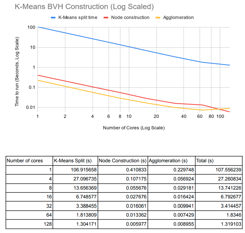
- We are also looking into the paper "Parallel BVH Construction using k-means Clustering" from the authors Daniel Meister and Jiri Bittner. We plan on visiting their approach and seeing how this approximate method using k-means will lead to more speed ups.
Goals and Deliverables - Plan to achieve
- Implement a fully functional parallel BVH creation pipeline that can be used for ray-tracing in Scotty3D
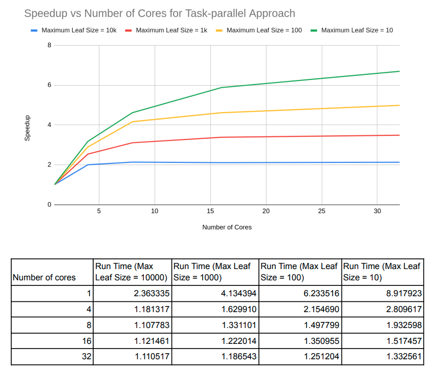
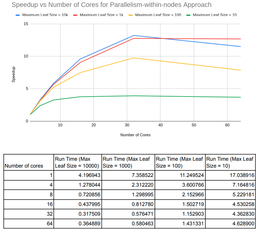
- Provide speed-up graphs for BVH creation on multi-core CPU platforms
- Provide speed-up graphs relative to BVH quality - BVH quality can be measured by SAH or rendering speeds
Goals and Deliverables - Hope to achieve
- Implement parallelism using k-means, which involves parallelizing the k-means algorithm
Platform Choice
- Written in C++ with message passing using OpenMP
Schedule
| Week | Goals |
|---|---|
| Week 1 | Revisit Scotty3D code and familiarize ourselves with how BVH creation works and plan out how our parallelization strategy will work |
| Week 2 | Implement parallelism for basic BVH creation for arbitrarily large scenes |
| Week 3 | Evaluate parallel algorithm in terms of BVH quality and speed-up achieved |
| Week 4 | Project checkpoint - Investigate other methods for BVH creation speed-up, e.g. k-means method |
| Week 5 | Implement new methods, e.g. k-means method and evaluate their performance with regards to speed-up and quality of BVH |
| Week 6 | Handin and Demo |